I recently wanted to refresh my memory about Machine Learning methods. I have spent some time reading tutorials, blogs and Wikipedia. No doubts, the Internet is really useful, this is great. I got back on tracks quickly with the general idea of the mainstream algorithms. However, from time to time, I find some particular points and explanations obscure. This concerns often details about the algorithms which are overlooked. Sometimes, the emphasis is on the main part of the algorithm and some details are left missing. But I found these missing parts quite important to fully understand what’s going on in the algorithm.

In this series of blog posts, I want to clarify or at least provide a different explanation of some of the concepts in machine learning, in the hope of helping people increase their understanding of these methods. Since I have spent quite some time studying the concept of entropy in academia, I will start my Machine Learning tutorial with it. Evaluating the entropy is a key step in decision trees, however, it is often overlooked (as well as the other measures of the messiness of the data, like the Gini coefficient). This is really an important concept to get, in order to fully understand decision trees.

Metaphoric definition of entropy

Entropy is a concept used in Physics, mathematics, computer science (information theory) and other fields of science. You may have a look at Wikipedia to see the many uses of entropy. Yet, its definition is not obvious for everyone.

Plato, with his cave, knew that metaphors are good ways for explaining deep ideas. Let try to get some inspiration from him. I like the definition of entropy given sometimes by physicists:

Entropy is a measure of disorder.

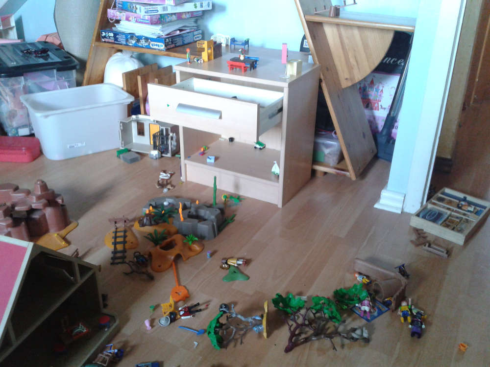
So let us take this point of view and think that our dataset is like a messy room:

Entropy is an indicator of how messy your data is.

Imagine you are about to tidy your room or your kids’ room. Usually, you use a subjective measure to estimate how messy is it. (not everyone has the same measure :), but this is not the topic here). You know that objects must be on the shelves and probably grouped together, by type: books with books, toys with other toys …

Fortunately, the visual inspection can be replaced by a more mathematical approach for the data. A mathematical function exists for estimating the mess among mathematical objects and we can apply it to our data. The requirement of this function is that it provides a minimum value if there is the same kind of objects in the set and a maximal value if there is a uniform mixing of objects with different labels (or categories) in the set.

Why entropy in decision trees?

In decision trees, the goal is to tidy the data. You try to separate your data and group the samples together in the classes they belong to. You know their label since you construct the trees from the training set. You maximize the purity of the groups as much as possible each time you create a new node of the tree (meaning you cut your set in two). Of course, at the end of the tree, you want to have a clear answer.

“To which group does this sample belongs to? Based on this arrangement of features, without doubt, it belongs to Group 1!”

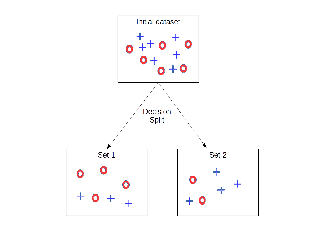
On the figure below is depicted the splitting process. Red rings and blue crosses symbolize elements with 2 different labels. The decision starts by evaluating the feature values of the elements inside the initial set. Based on their values, elements are put in Set 1 or Set 2. In this example, after the splitting, the state seems tidier, most of the red rings have been put in Set 1 while a majority of blue crosses are in Set 2.

So decision trees are here to tidy the dataset by looking at the values of the feature vector associated with each data point. Based on the values of each feature, decisions are made that eventually leads to a leaf and an answer.

At each step, each branching, you want to decrease the entropy, so this quantity is computed before the cut and after the cut. If it decreases, the split is validated and we can proceed to the next step, otherwise, we must try to split with another feature or stop this branch.

Before and after the decision, the sets are different and have different sizes. Still, entropy can be compared between these sets, using a weighted sum, as we will see in the next section.

Mathematical definition of entropy

Let us imagine we have a set of items. These items fall into two categories, have Label 1 and have Label 2. As we have seen, to get our data a bit more ordered, we want to group them by labels. We introduce the ratio

The entropy of our set is given by the following equation:

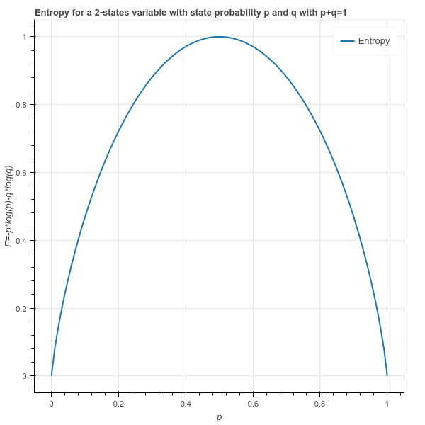
A set is tidy if it contains only items with the same label, and messy if it is a mix of items with different labels. Now have a look at the Entropy function, below. When there is no item with label 1 in the set (p=0) or if the set is full of items with Label 1 (p=1), the entropy is zero. If you have half with Label 1, half with Label 2 (p=1/2), the entropy is maximal (equals to 1 since it is the log base 2).

In addition to these properties, the function is symmetric with respect to p=0.5: among the two categories to classify, there not one which is messier than the other.

This function quantifies the messiness of the data.

Evolution of entropy

The entropy is an absolute measure which provides a number between 0 and 1, independently of the size of the set. It is not important if your room is small or large when it is messy. Also, if you separate your room in two, by building a wall in the middle, it does not look less messy! The entropy will remain the same on each part.

In decision trees, at each branching, the input set is split in 2. Let us understand how you compare entropy before and after the split. Imagine you start with a messy set with entropy one (half/half, p=q). In the worst case, it could be split into 2 messy sets where half of the items are labeled 1 and the other half have Label 2 in each set. Hence the entropy of each of the two resulting sets is 1. In this scenario, the messiness has not changed and we would like to have the same entropy before and after the split. We can not just sum the entropies of the two sets. A solution, often used in mathematics, is to compute the mean entropy of the two sets. In this case, the mean is one. However, in decision trees, a weighted sum of entropies is computed instead (weighted by the size of the two subsets):

where and are the number of items of each sets after the split and and are their respective entropy. It gives more importance to the set which is larger (if any). The idea is that it is a bit better if the large set gets tidier, as it requires more efforts to tidy. Imagine the worst case where a set of 1000 elements is split in two, with a set of 999 elements and a set of 1 element. The latter set has an entropy of zero since it contains only one element, one label. But this is not really important as the vast majority of the data is still messy in the larger set. So the two sets should be given importance relative to their size.

Limits of decision trees

Since it goes step by step, decision trees may not provide the optimal classification. It minimizes the entropy at each step but has no global view on the optimization process. Let me explain this differently. Sometimes it may be more efficient to start to put in order the bigger items in a room, even if there are not many of them and the impression of tidiness does not increase much after. You could then put the smaller items on top of the bigger to get a nicer view of your room. Starting the other way round might not lead to a room as neat. With the decision tree approach, you could also end up with many small groups of toys put in different parts of the room. They would be perfectly matched together however it would be better to group all the toys in one part of the room. This step by step approach is called a greedy approach.

Generalization

If you have more than 2 labels, you can generalize the Entropy formula as follows:

where the are the ratios of elements of each label in the set. It is quite straightforward!

You may use different kinds of entropies, have a look at Renyi entropy. It is a generalization of the standard entropy (Shannon’s entropy). I am not sure it is of interest for decision trees but it shows the general properties required to call a function “entropy”.

Conclusion

We have seen that entropy is not just a mathematical formula. It has a simple interpretation that everyone can understand.If you now see what is entropy you should have a clearer idea of what are doing decision trees.

By using entropy, decision trees tidy more than they classify the data.

In physics, the second law of thermodynamics states that the entropy always increases over time, if you don’t bring (or take) any energy to the system. Don’t wait too long before tidying your room or your data!

I hope you have found this post useful. More Machine Learning posts should come soon.