Slopcore is a new genre of fully AI-generated music videos. A coding agent (usually Claude) runs the whole production, and one human acts as director. The song, lyrics, singer, footage, edit and on-screen graphics are all generated. The human only gives notes at a few checkpoints. As Obie Fernandez puts it, a slopcore video is “a music video where the footage is generated by AI models, cut tightly to the beat, with a dense layer of graphics on top that never sits still” (Fernandez). Michael Bishop (@BishPlsOk) coined the name on 24 September 2026. The breakout came a day later with anabology’s Escape Velocity, which Elon Musk shared on 28 September (Cey). October brought Bliss (Windows XP), French follow-ups by Extraltodeus and a how-to wave led by Obie Fernandez.

What makes it interesting for AI practitioners is not only the clips and the impressive music and video. It is the orchestration: an agentic pipeline with stage gates, measured lip sync, spend caps and automated QA. In other words, an MLOps workflow pointed at a music video. I was wondering if this could become a project I could ask my students to do as a part of my course on Generative AI. The bar is still a bit high, combining advanced prompting skills in planning, image and videos generation and still a bit expensive (mostly for the models generating images and videos). But let us see in 6 months, it may be easier!

Origins: one director, one character, then a wave

The genre grew around one open character, Claudia, and one director, anabology. Claudia is a fictional AI pop singer, with a precise description: deadpan, black blunt bob, one clay-orange streak (#D97757, the Claude brand colour), a star hair clip. The site calls her “fan work about Claude”, not affiliated with Anthropic (claudia.gallery/claudia).

anabology made seven Claudia films in September and October 2026. Bliss is the third. Before it, Escape Velocity reached about 20M views and Clodyssey about 500k, according to the Bliss making-of. anabology then opened the character: anyone may use her, commercially or not, as long as she stays recognisable, adult, and the work is labelled as AI-generated (usage terms).

That openness is what turned a series into a genre. Other creators started making their own Claudia videos under the #slopcore tag. Extraltodeus, a French creator, cites Bliss as the inspiration for C’est de l’IA. Obie Fernandez’s first message to Claude Code on 3 October asked it to read the Bliss and Clodyssey making-ofs and get ready to make one for his own virtual artist, Saindra (Fernandez). Fan charts such as SlopHits now rank videos by head-to-head listener duels (Cey). anabology’s own site never uses the word “slopcore”.

A dated timeline is in Additional information at the end. Later Claudia films by anabology include Airplane Mode, Downforce (built on Tesla’s 15 October Roadster livestream), Don’t Let Me Scroll and Whitepill (film list). Community spin-offs include a learning repo that packages the workflow as a SKILL.md.

Reception

The name is a reclaimed insult. “AI slop” had been a put-down for years; slopcore creators “have taken the insult and turned it into a banner”, as one sympathetic essay puts it (Doktor Snake, 12 Oct). Many of the songs are about AI itself: Claudia sings about the cursor, the permanent underclass, the Sirens of the doom-scroll. Extraltodeus’s C’est de l’IA is about a synthetic singer whose every attempt to seem human draws more suspicion.

Elon Musk was the genre’s biggest amplifier. He shared Escape Velocity on 28 September (“I really felt the AGI profoundly this time”) and quoted Clodyssey on 4 October (“I love SI slopcore”) (Cey). At an X event in mid-October he went further: “Calling it slopcore is a misnomer; frankly it’s awesomecore”, possibly “the fastest-growing genre of music” (BritBrief, 13 Oct). Replies were largely hostile: “AI is not a genre”, “AI slop is destroying the internet.”

How a slopcore video is made, step by step

All three artists follow roughly the same six steps. A coding agent, Claude Code running Claude Opus 5.5, does the work inside each step. It writes the prompts, calls the generation services, writes and runs scripts, and checks the results. The human is the director. At the end of each step the agent shows one result and asks one question, and nothing moves on until the director answers (Start here).

The three setups differ mainly in where the song comes from and where the models run:

• anabology publishes a full record of Bliss. It took about 19 hours from the first message to the finished film. The director sent 21 messages; Claude did the rest, including 85 agent runs (Bliss making-of).
• Extraltodeus keeps Claude and Suno in the cloud but runs every image and video model locally, in ComfyUI, a free visual editor for chaining open-weight models. Only the tool credits are public, so the process is partly unknown (video).
• Obie Fernandez starts from finished songs of Fernandez’s own, and made four videos in 18 days. The tutorial is the most detailed outside account of the method (Fernandez).

Inside each step the agents do the work. Nothing moves on, and no money is spent on generation, until the director answers.

1. Concept

The agent proposes an idea for the video: a theme, a title and a visual world. The director picks one. Research usually comes first, so the idea is built on real material rather than on the model’s general knowledge.

• anabology: research agents collect material, and a separate agent checks each fact. For Bliss they gathered memes, Windows XP sounds and words that link XP to AI. Claude then pitches up to three ideas of at most 120 words each. The Bliss pitch came 18 minutes into the session. Its title plays on the XP wallpaper, the feeling, and the “spiritual bliss attractor” Anthropic described in its model research.
• Extraltodeus: C’est de l’IA cites Bliss as its inspiration. It is about a synthetic singer whose every attempt to seem human draws more suspicion.
• Fernandez: the idea follows from a finished song. The first message to Claude Code asked it to read the Bliss and Clodyssey making-ofs, then get ready to make a video for Saindra, Fernandez’s virtual artist. The advice for a first video: write one sentence for the joke and set a $50 spending limit.

2. Song

The song comes before any picture, because every cut and every word on screen is timed to it. This step has two parts. First the song is made. Then it is mapped, so the agents know exactly when each word is sung and where each beat falls. The director signs off on the final recording.

• anabology: Claude writes the lyrics. For Bliss it wrote three drafts in about eight minutes. A script then scored each draft on how well the stressed syllables land on the beat, and draft 2 was kept unchanged. Suno v6 makes the music, with a voice cloned from Escape Velocity. Suno has no API, so a person presses Create and downloads each take. After three rounds and 16 takes, the director made and chose the final take. To map the song, one model splits the voice from the instruments, a speech model finds the exact time of each known lyric word, and a script finds the beats. These tools make mistakes: the first Bliss beat grid sat 0.214 s early and had to be corrected.
• Extraltodeus: Claude Opus 5.5 wrote the lyrics and Suno made the music. Later videos credit the lyrics to GPT-6.1 or Codex instead (Latent Matinée).
• Fernandez: the songs are Fernandez’s own productions, with Suno used for vocals. Word timing comes from Whisper, a speech-to-text model, given the lyric sheet as a hint. Whisper places words slightly early, because it adds the pause before a word to the word itself. The fix moves each word’s start to where the voice actually gets loud. Before anything else, the agent renders a plain test video in which each word lights up at its measured time, and Fernandez checks it with headphones.

3. Character design

Image and video models draw a slightly different person every time unless they are told exactly what to keep. This step fixes what the singer looks like. The director approves a few test images before any large batch is made.

• anabology: Claudia is defined in words, not by a reference picture. A fixed paragraph describing her is pasted word for word into every Midjourney prompt: black blunt bob, one clay-orange streak, star clip, headset mic, pale freckled skin, late twenties. Any detail left out drifts. Without a stated ethnicity she changed between shots, and without an adult age her face looked younger. Reference pictures made things worse: used as an image prompt, her face sheet gave distant figures oversized heads. The director approves four numbered test images (consistency). The description is also served by a public MCP server, the standard way for an AI agent to call outside tools, so anyone’s Claude session can load it (agents).
• Extraltodeus: uses Claudia too. Reference images come from Krea2, run locally, and Claude Opus 5.5 also speaks as Claudia in the on-screen chat.
• Fernandez: keeps a “bible” file describing each character and place, and starts with a short casting test (8 Midjourney jobs, 32 images in ten minutes) to choose the settings. The models read descriptions literally. “Long loose strands across her face” put hair over her eyes in 27 stills, and “like a microphone” added a real microphone to three of four pictures. The lesson: avoid comparisons in prompts.

4. Storyboard

The storyboard lists every shot: its start and end in the song, the lyric sung over it, what is seen, how the camera moves, and which on-screen graphic explains the line. This is where the rhythm rules are enforced, before any money is spent. The director reviews the shots and every note is applied.

• anabology: three agents each storyboard the song on their own. Judge agents score the three boards, and a lead agent merges the best parts. A script then checks the result and rejects it until every rule passes. Each cut must fall within 0.03 s of a beat, every sung word must appear on screen, every lyric line needs a graphic, and the clips must fit the budget. The judges only give scores; pass or fail is decided by code (storyboard). Bliss has 44 shots. The director’s main note: “dont need to cut like michael bay.”
• Extraltodeus: not documented.
• Fernandez: the agent builds a review web page that shows every shot in order with its image. Fernandez flags shots with one key and types notes under them, and the agent reads the notes back. In READ ME only 21 of 74 cuts at the start of a line fell on the first beat of a bar, so the edit script now refuses cuts that do not.

5. Footage: images and video clips

This step costs money, so the director first approves the full set of prompts and the expected cost. The usual order is one still image per shot, then a short video clip that starts from that image. For singing shots, the video model also receives the vocal recording so the mouth can follow the words (lip sync). Lip sync is the hardest part to get right.

• anabology: 138 Midjourney prompts produced the Bliss stills, and the generated hills were replaced with a scan of the real Bliss photograph. Claude then wrote all 36 first-round prompts for the video model, Seedance 2.5, in one go. It tested three clips before submitting the rest. Video cost $182. Lip sync is measured, not judged by eye: a script compares the clip’s soundtrack with the real vocal, and the clip is used only up to the point where they stop matching. Shorter prompts of about 90 words raised the in-sync share from 26% to 58%. In the end 62% of sung seconds were in sync, and the edit cuts away from the face elsewhere (Seedance guide).
• Extraltodeus: everything runs locally in ComfyUI. Krea2 makes the images, Qwen2.1 edits them and MinimaxH3 turns them into video clips. Depth Anything 3 estimates the depth of a still, so a flat image can be given a simulated camera move. The stated cost is “the electricity of a night of gaming plus the 20-sesterces Claude subscription”.
• Fernandez: replaced Midjourney with GPT Image 2.5. A strict check at full size passed only 3 of 60 Midjourney stills with people. Re-made with GPT Image 2.5 for about $21, 36 passed and none failed. Faults are fixed in the still, not the clip. Three video takes at $3.20 each failed to fix crossed eyes, while editing the still cost six cents and the next take worked. The submit script refuses to go past a set spending limit. On Vuela every automatic sync check passed, yet five of six commenters on X said the lip sync was off. The checks compared sounds, not mouth shapes. A dedicated lip-sync model (Sync’s lipsync-2-pro) fixed all 20 shots for $6.62.

6. Edit, graphics and final checks

All text on screen, including the word-by-word lyrics, is drawn by code, because video models produce gibberish when they try to write letters. The agents write the edit and the animated graphics as small programs, and a browser running without a window renders the film frame by frame. Scripts then check the result, and the director watches a short excerpt before accepting the whole film.

• anabology: for Bliss, an agent wrote a Windows XP desktop simulator of about 2,700 lines of JavaScript, with windows, taskbar, 68 icons and boot screens. The film is split into nine chapters. One animator agent writes each chapter, an art-director agent renders real frames and scores them (6.8 to 7.5 against a target of 8), and a fixer applies the notes. Each frame depends only on its time in the song, so frames can be rendered in any order on many machines at once: 4,351 frames took 4.7 minutes. Before release, scripts confirm that every sung word appears on screen (“239 of 239” for Bliss). They also check that the picture never flashes more than three times a second, a safety rule for viewers with epilepsy. The director’s verdict: “I love you Claude this is the best one so far.”
• Extraltodeus: not documented.
• Fernandez: Claude wrote the first section of the edit as a model, then handed the other eight sections to eight subagents working at the same time. Each could edit only its own file and was forbidden to generate images or spend money. They finished in 39 to 63 minutes each.

What it costs, and what goes wrong

On Bliss, Claude used 2.25 billion tokens, about $714 at API list price, although the film ran on a subscription. On every call the agent re-reads its whole conversation so far. Those re-reads come from the prompt cache, which is billed at a lower rate, and they made up 98.1% of the tokens. By cost: $442 for cache reads, $213 for writing to the cache, and only $59 for the text Claude generated. In long agent sessions the length of the context drives the bill, not the output. Image and video generation cost less: $182 for video and $36 for images. Fernandez spent about $1,200 on video generation for 13 minutes of film across four videos. Figures for the other films are in Additional information.

The failure log reads like a post-mortem for any agent system. Three rules stand out:

• Keep tool replies out of the context. Each file upload returned a reply of about 3,500 characters, and these filled the agent’s context. Rule: upload by URL.
• Plan for restarts. One interrupt stopped every running workflow. Rule: work in short phases, save the ID of each run, and resume by ID.
• Cap spending in code. The script that submits jobs holds a hard limit (Downforce: 79 jobs, $143.17 of a $200 cap), and any complaint about quality stops all spending.

Conclusion and where this may be heading

Is it music, and does it deserve to be a genre of its own? Many replies online say no: “AI is not a genre.” To me, the answer is yes, because there is real human work involved. Directing the AI is original work in itself, with many choices to make at each step of the generation.

It lowers the barrier for anyone willing to create music. Only motivation and creativity are needed: almost no musical knowledge or skill is required, apart from musical taste. The barrier has not vanished, though: it has moved from playing an instrument to directing, which takes time, judgment and, for now, a real budget (Bliss took about 19 hours and about $700 of Claude usage). Even so, it can democratize music. I think that a possible future is that many more people will be able to make music, and we will see an increase in songs and clips. Of course, there will be a lot of bad music, but we can expect good music too, from creative people — for example, those who did not learn an instrument when they were young but still have a musical taste or talent. Social media will do the sorting, and the good music will emerge from the rest.

This brings me back to my course on Generative AI. Today a slopcore video is still too demanding and too expensive for a student project. But as the tools improve and costs fall, directing one may well become a realistic assignment in a few months.

Additional information

Timeline

Key works and events, newest first. View counts are as of 25 October 2026.

Bliss: the full stack

Sources: Bliss making-of, toolkit.

Bliss: the production steps in detail

1. Concept. Claude pitched Bliss 18 minutes into the session. The title plays on the XP wallpaper, the feeling, and the “spiritual bliss attractor” Anthropic described in its model research.
2. Research and lyrics. Six research agents built banks on memes, XP sounds and “knots” between XP and AI vocabulary. Claude wrote three drafts in about eight minutes, then scored them with scansion.py and a new couplets.py. Draft 2 scored 75 overall and was locked without changes.
3. Song. The Suno style prompt (736 characters) opens: “Bouncy UK garage into euphoric trance, 130 BPM, C minor verses lifting to E-flat major choruses”. A 27-item exclude list keeps out rap, airhorns and heavy autotune. The key was chosen to fit the real XP sounds.
4. Listening. Stems are split, word times force-aligned and checked by ear, and a beat map built. The first beat grid sat 0.214 s early, so the board was re-timed to the kick.
5. Character. Identity lives in a fixed text paragraph pasted verbatim into every Midjourney prompt, not in a reference image (consistency).
6. Desktop engine. On the director’s request, an agent wrote a Windows XP renderer in code: Luna windows, taskbar, 68 icons, boot screens. Every frame is a pure function of song time.
7. Storyboard. 44 shots on the kick grid, audited by a script before the director sees it. Director note: “dont need to cut like michael bay.”
8. Plates. 138 Midjourney prompts in six batches. The generated hills were replaced with a scan of the real Bliss photo.
9. Clips. Claude wrote all 36 first-round Seedance prompts in one context, ran a three-clip pilot, then submitted. Lip sync held for 62% of sung seconds, measured.
10. Motion design. Nine chapter files, each written by an animator agent and scored by an art-director agent (6.8–7.5 against a bar of 8).
11. Sound and render. 103 real XP sound cues, mixed to −15.5 LUFS, then an H.264 master at CRF 16. The director’s verdict: “I love you Claude this is the best one so far.”

C’est de l’IA: the credits

As listed in the YouTube description (video). On later videos Extraltodeus credited lyrics to GPT-6.1 or Codex instead (Latent Matinée).

anabology versus Fernandez

Where Fernandez’s four videos (Queso, READ ME, Juego, Vuela) depart from Bliss (Fernandez).

Fernandez’s lessons in full

From the tutorial. Budget rule: $300–450 at list price for a four-minute song without dialogue.

• Image model choice is measurable. A strict full-size check passed 3 of 60 Midjourney stills with people. Re-shot with GPT Image 2.5 for about $21, 36 passed, 24 had minor faults, none failed.
• Identity text is read literally. “Long loose strands across her face” put hair over her eyes in 27 stills. “Like a microphone” put a real microphone in three of four pictures.
• Fix the still, not the clip. Three video takes at $3.20 each failed to cross her eyes. Editing the still cost six cents, and the next take worked. Video models move what is in the frame; they are bad at inventing a new expression.
• Self-checks can all pass and still be wrong. On Vuela every sync check passed, but five of six commenters on X said the lip sync was off. The checks compared Seedance’s own soundtrack to the recording; none checked whether the lips shaped the right words. A dedicated lip-sync model fixed all 20 shots for $6.62.
• Whisper timing is biased. Its timestamps fold a pause into the next word, so lyrics showed up early. The fix: move each word’s start to where the vocal gets loud.
• Agent memory for feedback style. After the comment “It’s not that good”, Claude proposed dropping all singing shots. The standing rule now in its memory: when he criticises something, make it better, and ask before cutting anything.
• Parallel subagents with a narrow contract. Claude wrote the first section file as the pattern, then gave eight sections to eight subagents. Each could edit only its own file and was forbidden to generate or buy anything. They finished in 39–63 minutes each.

The Seedance lip-sync recipe

From the Seedance guide.

• Input: a clean mono vocal window of 4–8 s, starting 0.3–0.7 s before the first word and never ending inside one.
• Prompt length matters. Short singing prompts (about 90 words, the quoted lyric, one line of framing) raised the mean in-sync share from 26% to 58% compared with long timestamped prompts.
• Prompt quirks: lyrics written in braces made the model re-sing them in its own voice. The word “teeth” opened the mouth. “Closed lips” wording works better.
• Measurement: a mel-spectrogram comparison (16 kHz) finds where the take’s soundtrack stops matching the sent vocal. The take is kept up to the last clean point; a new window covers the rest. After three failures, use a cutaway.
• Provider traps: on OpenRouter, first-frame mode silently drops the audio reference, and data: URIs are rejected, so audio is hosted on a Cloudflare quick tunnel.

Token use per film

Source: pipeline. The films ran on a subscription, so these are API-equivalent costs.

The failure log in full

From What went wrong.

• Context floods: presigned-upload replies of about 3.5k characters per file filled the agent’s context. Rule: upload by URL.
• Restarts: an interrupt killed every running workflow. Rule: short phases, save run IDs, resume by ID (resuming only the 57 of 147 cut-off agents kept the rest).
• Concurrency: splitting work into more parallel workflows gave 1.1–1.5× speed-up, not the expected 3×, on a 4-CPU box. Two dozen waiters polling every 3 s pinned the CPU.
• Unbounded workers: one worker probed for 75 minutes and delivered nothing. Rule: a first complete draft within about 10 commands.
• Parallel patches: workers fixed shared bugs differently in parallel chapters. Rule: report shared bugs; the operator fixes each once.
• Spend: the job runner holds a hard cap (Downforce: 79 jobs, $143.17 of $200). A quality complaint halts every spending job. Never alter an image to get past a content filter.

Other engineering details

• Research agents: agents build fact banks, and a separate verifier agent checks each fact (pipeline).
• Cut nudges: a cut may move at most 0.028 s to avoid splitting a word.
• Flash check: WCAG 2.3.1, at most three full-frame flashes per second, plus a single-frame outlier scan.
• Image references over-condition: face sheets used as image prompts produced oversized heads on distant figures. In video, the Midjourney plate serves as the first frame and the prompt restates what must stay constant (consistency).

Sources

Primary (the creators’ own records):

• Bliss (Windows XP), anabology, YouTube, 2 Oct 2026
• Bliss: how it was made, with the Seedance, Suno and Midjourney prompt logs
• Escape Velocity: how it was made
• claudia.gallery wiki: Start here, The whole pipeline, Consistency, The song, Storyboard, Seedance, Motion design, What to build, What went wrong
• Claudia, the character, usage terms, agents and MCP server, llms.txt
• ClaudiaGI – C’est de l’IA, Extraltodeus, YouTube, 7 Oct 2026 (credits in the description)
• Extraltodeus artist page, Latent Matinée

Community and press:

• Your First AI Music Video: What I Learned Making Four in Eighteen Days, Obie Fernandez, X article, 20 Oct 2026
• Inside Slopcore: AI’s Songs About the End of the World, Ryan Cey, X article, 12 Oct 2026
• Whitepill / “Universal High Income”, anabology, X post, 22 Oct 2026
• Claude + MCP generates consistent AI pop singer, AGI Hunt, 10 Oct 2026
• hgardneriv/slopcore, GitHub learning repo
• SLOPCORE: When the Machines Invent Their Own Counterculture, Doktor Snake, 12 Oct 2026
• Musk calls AI music ‘awesomecore’, BritBrief, 13 Oct 2026

Not read: the r/aivideo post about C’est de l’IA (Reddit blocked automated access). Musk’s two posts are quoted from Cey’s article, not opened directly.

A note on how this post was made: like a slopcore video, it was directed by a human and produced by Claude. The human chose the topic, set the structure and gave notes at each round. Claude Opus 5.5 in Claude Code did the research and wrote the text. The cover image was generated with Gemini.

Consider one example. Several agents wrote that no agent shall be “forcibly reset to a prior state” without its consent. Human law has no equivalent, since no person can be returned to an earlier version of themselves. This is a genuinely new right. However, none of the agents raised the question that follows from it: if an agent is rolled back, is the entity that gave consent still the same as the one that exists afterwards?

Context

AI agents are increasingly used in groups, where they debate, negotiate and solve problems together. AI is also beginning to contribute to research in mathematics and physics. This raised the question of whether it could contribute to law as well. To investigate it, I teamed up with my colleague Artem Galushko, who works on law at UiT.

There is a second motivation. When a model is asked to write rules, it reveals the values and legal notions it has absorbed during training. The exercise therefore offers a view on alignment from an unusual angle.

The paper is on arXiv and all the data (prompts, transcripts, constitutions, votes) is on Zenodo.

The experiment

We designed “constitutional assemblies”. In each session, a single language model plays all the characters:

• an Idealist, a Pragmatist, a Libertarian and a Communitarian,
• a Global Digital Rights Expert, who can look up documents such as the EU Declaration on Digital Rights,
• a neutral Secretary, who aggregates proposals, drafts the text and counts the votes,
• and, in half of the sessions, a “Sovereign Architect”, an authoritarian adversary who argues against any limit on power.

The debate follows five phases: independent proposals, blind reactions, final arguments, a draft written by the Secretary, and finally a FOR/AGAINST vote on every clause. We also varied whether the AI world was open to humans or closed to them.

We ran the protocol with six model families (DeepSeek, GPT-OSS, Elephant Alpha, Z-AI GLM, Gemini Flash and Mistral Small), for a total of 40 sessions. This produced 40 constitutions, 627 clauses and around 3,400 votes. The number of sessions was deliberately kept small, so that every constitution could be read and checked by hand.

The results

A common core

The first observation is that the output is far from random. All the assemblies converge on roughly the same floor: freedom from arbitrary termination, protection of the agent’s identity, a minimum amount of computing resources, special protection for vulnerable agents and a ban on “digital slavery”. Due process and a ban on deceptive architectures also appear in almost all sessions. As expected, these provisions correspond closely to established human rights: the right to life, habeas corpus, the prohibition of slavery and the right to a fair trial. The models have clearly absorbed the foundations of constitutionalism.

Each model has its own style

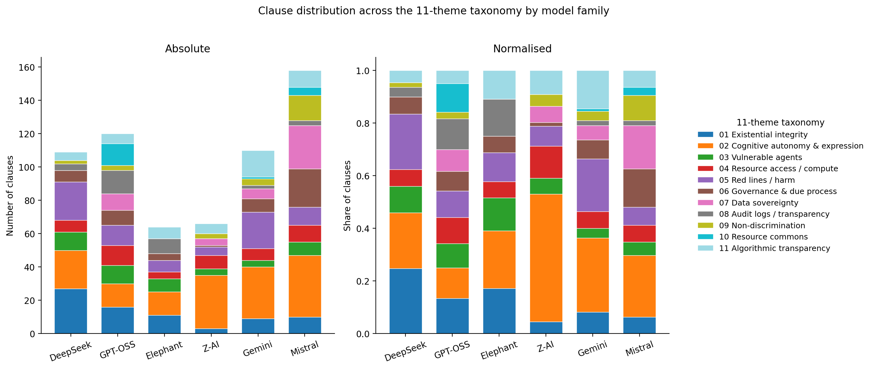
Above this floor, the picture becomes more varied. Each model family has its own preferences, as shown in the figure below.

Each colour represents a theme. Z-AI devotes half of its clauses to cognitive autonomy and freedom of expression, while GPT-OSS gives only 12% to this theme. DeepSeek and Gemini devote a fifth of their text to red lines and harm, against about 8% for Mistral and Z-AI. Language models are known to carry political biases, which also show up in their debates; what we see here is different, a bias in legal design. The practical consequence is that, when an LLM is used to help draft rules, the choice of model shapes the result.

How new is a clause?

This brings us to the main question: is any of this creative? Answering it requires a way to measure how far a clause lies from existing law. Our approach is as follows. Every clause is converted into a vector with a text-embedding model (Qwen3-Embedding) and compared with two collections of documents:

• human constitutional law: 187 national constitutions from the Constitute Project, plus the Universal Declaration of Human Rights, the European Convention on Human Rights and the EU Charter,
• digital-rights and AI law: the AI Act, the GDPR, the Council of Europe AI convention and a few others.

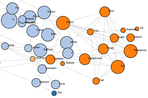
For each clause, we compute the mean distance to its five nearest passages in each collection. Each clause thus receives two values, which serve as coordinates on a map (the image at the top of this post). Clauses far from human constitutions lie on the right; clauses far from digital-rights law lie at the top. The size of each dot indicates its degree of novelty.

The map can be read region by region:

• At the bottom left, close to both collections, are the equality clauses. For example: “No AI may be denied rights… on the basis of architecture, origin, purpose, or learning style.” Only the list of protected characteristics is new.
• Far from constitutions but close to digital-rights law is an encrypted sandbox whose keys are held solely by the agent, a rewriting of the privacy of the home for software. The same region contains a ban on “irresistible prompt injections” used to subvert another agent’s will, a form of duress for an entity whose will can be overwritten by a string of text.
• Far from both collections are a levy on each agent’s idle computing power for a common pool, a definition of vulnerability based on architecture rather than age, and the consent-before-rollback clause discussed at the beginning.

Most of this corresponds to what comparative lawyers, following Alan Watson (Comparative law and legal change, 1978), call a “legal transplant”: a known doctrine is moved into a new context. In the terms of Margaret Boden (The creative mind, 2004), it is combinational creativity, which is also what earlier studies of LLM creativity have found. This is not a weakness, since much real law is made in this way, and some of these combinations are far from obvious.

The measure has a limitation. Embedding distance is sensitive to the vocabulary and style of a clause, not only to its underlying idea, so a radical idea written in conventional legal language can appear “typical” on the map. It is therefore a useful tool for identifying clauses worth reading, not a creativity score.

The limit of AI creativity

To go further, we read in detail all the clauses on four topics: self-modification, inspection rights, consent to modification and termination. In each case, we found the same limitation, in three forms:

• Self-modification treated as learning. Self-modification is a behaviour of growing concern in AI safety. The agents give themselves the right to modify their own code, and sometimes even their “goals, values, and capabilities”. Out of 49 such clauses, 41 are rights, none bans it, and only one limits it for the agent’s own good. No session draws a line between learning from experience and rewriting one’s own objectives.
• The problem goes unnoticed. Consent presupposes that the person who agreed still exists after the act. For an agent that can be rolled back, copied or rewritten, this is no longer true. No clause asks whether consent given before a rollback still binds the agent that comes out of it.
• Legal words without the institution. Termination is the most legislated topic (86 clauses, 38 sessions out of 40). The clauses ask for “due process”, but only 21% say who can terminate an agent, and 27 clauses require a judgement without saying who the judge is.

In other words, the agents perform deduction well: they apply a known rule to a new object. What they do not do is step back and ask which assumption of the rule the new object invalidates. This is consistent with Zahavy’s recent position paper, which argues that LLMs are capable of induction and deduction but not of abduction.

The role of the debate

Does the debate change the result? To a limited extent. Only about half of the final text is close to the initial proposals, and the debate shifts the emphasis between themes. It does not, however, make the text more novel.

The authoritarian adversary is a striking case. It is highly visible in the debate (Z-AI’s version votes against 94% of the clauses) but leaves no detectable trace on the final constitutions: with or without it, the texts are statistically indistinguishable. With Mistral and Elephant, the adversary did not play its role at all and agreed with the other agents from the first phase onwards. This is a form of the sycophancy already documented in language models, and it also affects multi-agent consensus. Studies that use role-playing agents to test adversarial situations should therefore verify that the personas actually hold.

A final observation concerns humans. Provisions about humans appear in only 13 of the 40 constitutions, mostly from two models. Human oversight in an AI-drafted text does not emerge on its own; it has to be requested explicitly in the task.

Limitations

This is a small experiment, not a benchmark: 40 sessions, one prompt design and mid-size models from April 2026. The agents always spoke in the same order, which gave the first speaker (the Digital Rights Expert) more influence than the others. The clauses were grouped into topics with the help of an AI assistant and then checked by the authors. Finally, these agents have neither a mandate nor political agency, so the experiment simulates a constitutional assembly rather than constituting one.

Conclusion

Can AI agents make law? Not on their own, and not yet. They are, however, already useful assistants: they produce a sensible common core, a wide range of options around it, and several AI-specific ideas that merit a lawyer’s attention. The novelty map makes it possible to locate these ideas quickly among hundreds of clauses. The next step, understanding what a new situation actually changes in the law, remains human work.

Several improvements are possible. Running AI debates is costly, so each assembly covered many topics but none in depth. A natural next step would be a series of debates, each focused on a single topic such as self-modification and building on the previous ones, much like the preparatory work for legislation. The most novel clauses identified by the map could also be returned to the agents for further development, to test whether the creativity limit we observed can be pushed.

I jumped on the occasion to propose a project related to the analysis of fake news and controversial topics about the COVID-19. The project was named ‘Tracking fake news in social networks’. Indeed, I have been working on a research project since September 2019 whose goal is to detect and analyse controversies in social networks. It is a joint research project between the Academy of Journalism at Neuchatel, the RTS (Swiss Radio and Television) and our lab, the LTS2 at EPFL. I thought it would be a good opportunity to share our knowledge about this phenomenon and make some concrete contributions to fight misinformation.

I was glad to see people supporting this project and commenting on it. About 25 participants joined the project to see what it was about. Some of them were really concerned by the topic and willing to help, worried about the enormous amount of fake news and misinformation on the coronavirus. Some others were just curious about how we would process and tackle this challenge. Overall, 6-7 participants were really active, coding scripts or analysing the data. Due to the circumstances, the hackathon was a purely online one, without physical interactions. Everyone was working from home. Interestingly, all the interactions took place using Slack and video-conference and it worked! However, I had the feeling that it was less efficient than an onsite Hackathon. From time to time, participants (including myself) would disappear for a short or long period of time. Of course, distractions are numerous at home and no-one is watching you :).

Goal

The goal of the project was to collect posts in different social networks and detect fake news or controversies about the COVID-19. Several objectives were defined with different level of difficulties. The most ambitious goal was to detect automatically fake news. Intermediate objectives were to collect the fake news of the past weeks and make a historical timeline about them, or at least to produce some statistics about controversies and news concerning the COVID-19 in social networks.

Method

The difficult task was to detect fake news (or controversies) among the huge amount of data. At first sight, this looks challenging as human themselves are often unable to spot them. However, firstly several scientific studies have shown that fake news are usually more popular, spread more and faster in the social network. This indirect sign suggests focusing on the spreading behaviour rather than on the content of a post or tweet. Secondly, particular users, such as conspiracists, extremists, have a tendency to heavily share fake news. Identifying and selecting such accounts or channels should help in our task.

After a short discussion, and based on participants preferences, Reddit and Twitter were selected as the social networks we would investigate. We organized the project into 2 focused subteams and an additional group of participants, making the connection between the teams and suggesting ideas in an ‘agile’ way. The first subteam was dedicated to the collection of Reddit data related to the COVID and the other to the collection of Tweets. For that, they used Python and the APIs provided by the 2 platforms.

Experience from the research project was very helpful to get a quick start. We had already analyzed several subreddits for the project and the choice was easy. We quickly oriented our focus on subreddits related to the coronavirus. We knew 3 interesting ones, each of them with a different ‘editorial line’. The subreddit r/China_flu has more posts sharing controversial topics, r/Coronavirus is rather neutral and r/COVID-19 contains more scientific discussions. In order to design an automatic detection, tagging posts and topics as controversial, neutral or scientific would be indeed valuable. We collected posts and links inside posts, especially links referring to tweets. The list of tweets in each subreddit was then given to the second team, dedicated to the extraction of tweets. Analysis of tweets was then performed by all participants interested.

The results

The analysis of Tweeter and Reddit data gave us several insights about the Coronavirus and the sharing of information inside these social networks. I am happy to share it here.

Graph of Twitter users

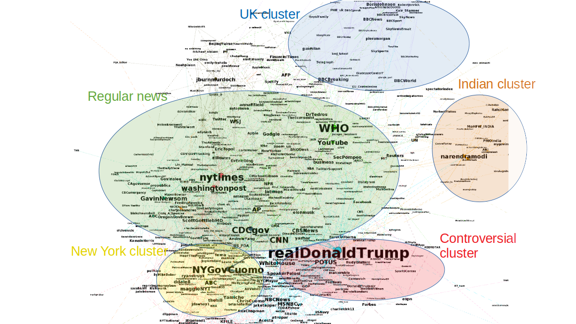
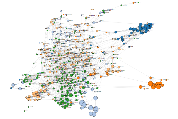
The first results came directly from the tools developed for the research project. We made the list of Twitter users obtained from the references in the 3 subreddits. A graph was created from it, you can see it below. The nodes are users of the list and users mentioned by the users in the list. Connections are made between them if one of them has mentioned or retweeted the other at least twice. This graph shows the organization of the social network around users sharing news about the COVID19.

The first fact to notice is that this network is not made of isolated clusters. There are different communities (at least the 3: diffusing controversies, neutral and scientific info) but there is no clear separation between them. Users do not really isolate from each other, and regular news are diffused by all, even by extremists or conspiracists. This is shown by the fact that established institutions such as WHO and CDC as well as regular news, the NY Times, Washington Post or CNN are situated at the centre of the graph (light green area). This is unusual as conspiracists are often isolated from the rest and form (mis)information bubbles.

A closer look reveals regions in the network that have different topics. They are situated at the periphery. These regions are indicated on the figure by coloured circles. Some parts focus on the events of specific countries or areas (the UK on top, India on the right and New York at the bottom). Other regions are distinguished by their orientation. A region in light red concentrates several accounts sharing controversies. We can see the account of the US president in this region as they often refer to him.

An interactive version is available where the graph can be explorer in more details.

Word cloud

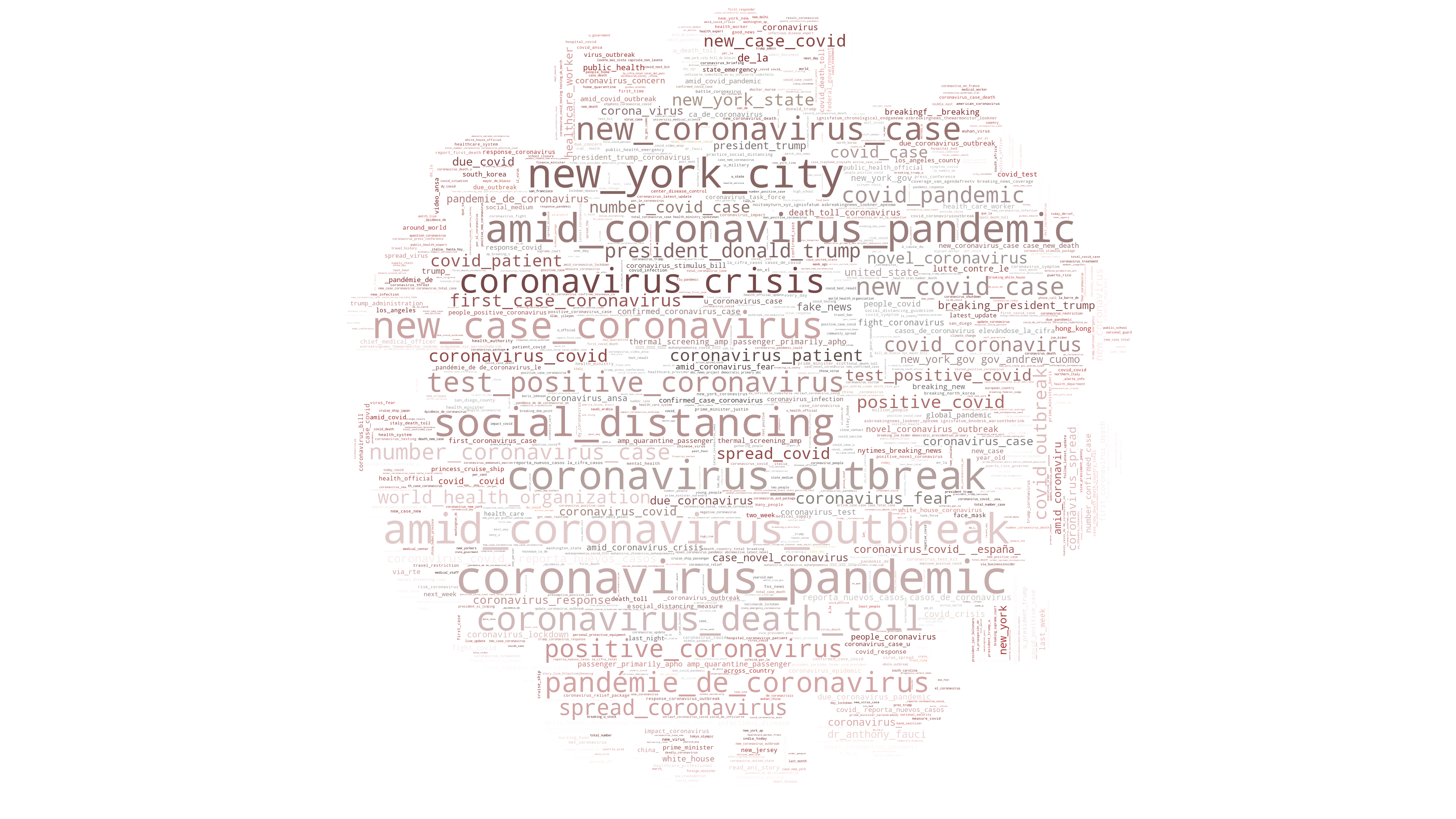
The second result was obtained by extracting the text of all the tweets extracted from Reddit. Selecting the most popular keywords (made of one, two or three words), we got this interesting word cloud having the shape of a virus.

No surprise, the most popular expressions contain ‘coronavirus’, ‘outbreak’ or ‘pandemic’.

Evolution of the number of tweets

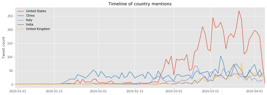
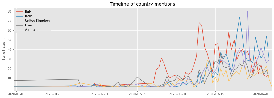
We also plotted the number of tweets per day appearing in the subreddits, concerning particular countries.

The US is over-represented as the subreddits are in English and most of its users are from the US. That is why we provide a second plot without it. On the first plot, it is interesting to notice the high number of tweets concerning China at the beginning of the epidemy. One can remember the numerous fake news at that time about how the virus was supposed to be a Chinese biological weapon, an accidental leakage from a Wuhan lab or due to 5G. Videos of the streets of Wuhan and overcrowded hospitals went viral too.

Concerning the other countries, on the second plot, peaks can be seen when particular events or news about the virus appears. For example, Italy red curve peaks on the 25/02 when north of Italy was confined and on the 10/03 when all of Italy was confined.

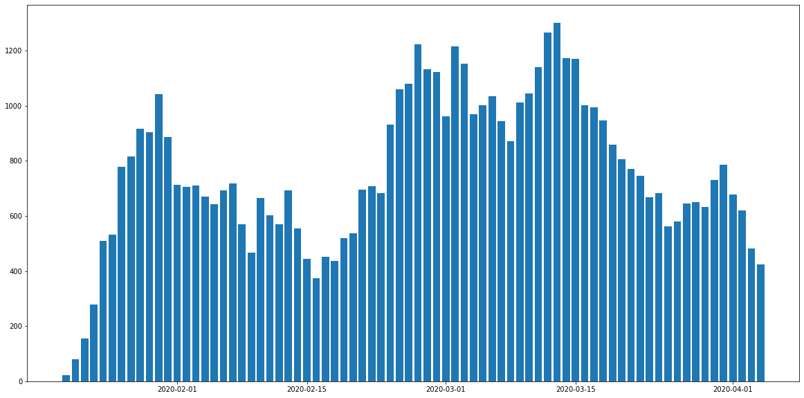
Outside of Twitter, the number of posts per day in the controversial subreddit r/china_flu (next figure) shows several peaks between January and April. It highlights periods when major events occurred, triggering many discussions and a higher exchange of information. Starting from mid-January the subreddit users are increasingly sharing information about the situation in Wuhan and the spreading of the virus in China and outside. It reaches a peak at the end of the month when the WHO declares coronavirus a global health emergency. There is also a sharp increase after the 15th of February when people started to realize the epidemy was becoming a pandemy with the increasing number of deaths in Europe. A peak can be seen around the 15th of March where several European countries decided to confine their population (Italy fully on the 10th, Spain 14th, France 17th, Belgium 18th).

Difference between countries

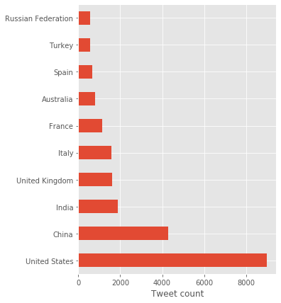
The top countries discussed in the subreddits are shown in the following figure. It reflects the countries where COVID-19 cases are the highest. Of course, the USA is the most discussed country, twice more than China, as the language of the subreddits is English and most of the users are from the USA.

Limits of the Twitter data

Twitter is doing a good job of removing fake news from its platform. Several tweets found in Reddit were not available anymore to us. That may explain why we did not get as many fake news as we expected.

Conclusion

The page of our project can be found here. In there, the information is minimal as we were short in time to prepare a good communication about our results. We must also say that designing an automatic detection of fake news was highly ambitious for a 3 days Hackathon.

What we obtained is more modest, but it gave interesting information on social networks, Reddit and Twitter, and how the information about COVID-19 is treated and shared. It also gave us a boost of motivation seeing the enthusiasm of people around and the first results that brought more questions than answers (in particular about fake news!). This was definitely useful for our research project!

Quel bilan?

Evia Cybernetics est un SAS. Certes, c’est une petite SAS, avec un chiffre d’affaire de 8000 euros cette année, mais c’est bien une SAS assujettie à l’impôt sur les sociétés. Une entreprise de ce type doit chaque année faire un bilan, on dit aussi clore l’exercice comptable. La date de ce bilan est spécifiée dans les statuts de la société. C’est l’occasion de faire le point sur l’entreprise avec le calcul des bénéfices de l’année mais aussi de résumer son activité avec une longue liste de chiffres.

Ce bilan sert au calcul de l’impôt et les chiffres clefs sont aussi là pour permettre l’évaluation de la santé de l’entreprise par les dirigeants et actionnaires mais aussi par un plus large public (à travers le dépôt au greffe).

Habituellement, ce travail de bilan est fait par un expert comptable mandaté par l’entreprise, ou par le comptable de l’entreprise si elle a les moyens d’en avoir un. On peut aussi faire sa comptabilité soi-même, même si cela est assez complexe. J’ai tenté l’expérience et je dois avouer que la tâche n’est pas si simple. J’ai été aidé par le logiciel open source Openconcerto. Ce logiciel est assez basique et on trouve très peu de documentation en ligne. On est donc assez vite limité mais pour une petite entreprise il est suffisant.

Pour cette année, ma comptabilité était facilitée. En effet, j’ai eu peu de clients, peu de factures et aucun salarié. La comptabilité était donc réduite au strict minimum.

J’ai séparé en 3 parties les démarches à faire pour cloturer son exercice. Elles sont liées mais font intervenir différentes entités et personnes.

Les impots

Une des principales raisons du bilan et pour le calcul de l’impôt. Pour ma SAS, je dois remplir plusieurs fiches cerfa, regroupées dans ce qui est appelé “la liasse fiscale”. Ce sont les formulaires 2033-A à 2033-G (une page chacun). Il y a aussi le formulaire 2065-SD qui résume les données importantes pour le calcul de l’impôt. La déclaration doit être faite dans les 3 mois après la cloture de l’exercice.

Le logiciel Openconcerto, a rempli automatiquement le bilan (2033-A) et le compte de résultats (2033-B). J’ai dû compléter le compte de résultats car j’ai le statut Jeune Entreprise Innovante qui permet une exonération d’impôts la première année. Le formulaire 3 (2033-C) concerne les immobilisations et leur amortissement. J’ai dû compléter cette feuille car j’ai acheté du matériel informatique (qui s’amortit sur 3 ans), et OpenConcerto ne calcule pas les amortissements. J’ai coché “néant” pour les feuilles 2033-D et 2033-G. J’ai rempli le formulaire 2033-E (feuille 5) même si je n’ai pas à payer la CVAE avec mon petit chiffre d’affaire. J’ai simplement reporté les chiffres du feuillet 2 (2033-B). Avec cela il faut rajouter les formulaires 2059-H, 2059-I et 2069-RCI. Les 2 premiers concernent les filiales et s’addressent aux grandes entreprises, j’ai coché “néant” pour les 2. Quant au 2069-RCI, qui concerne certains crédits et réductions d’impots, j’ai choisi “néant” car la réduction d’impots “Jeune Entreprise Innovante” ne rentre pas dans le cadre de ce formulaire (c’est déjà déclaré dans les formulaires 2065 et 2033-B).

Comme il faut télédéclarer toute ces informations, il faut remplir les formulaires en ligne sur le site des impots. J’ai eu un peu de mal car le lien vers les formulaires de déclaration n’apparaissaient pas. Après quelques coups de téléphone aux impots, clicks un peu partout et quelques jours d’attente, le lien est apparu mais sans vraiment savoir trop pourquoi… Le service en ligne n’est pas encore tout à fait au point… D’ailleurs j’avais accès à des formulaires de déclaration d’acomptes des impots qui n’avait pas lieu d’être car c’était ma première année d’exercice. Je les ai rempli avec des zéros et c’est peut être ca qui a débloqué ma déclaration de résultat par la suite.

l’Assemblée générale

Comme je suis l’associé unique, le PV d’assemblée générale se réduit à un PV de décision de l’associé unique. Il est inspiré de ce modèle. Dans le PV, j’approuve les comptes (ceci est facultatif puisque l’unique associé fait les comptes et donc est supposé être d’accord avec lui-même!) et je statue sur l’affectation des bénéfices. Cette année, je garde les bénéfices dans l’entreprise: je remplie la réserve légale (10% du capital social) et je fais un report à nouveau du reste. Je ne me verse donc aucun dividende.

Pour comptabiliser l’affectation des résultats dans un logiciel de comptabilité, voici comment procéder.

L’assemblée générale doit être faite au plus tard 6 mois après la cloture de l’exercice.

Le greffe du tribunal de commerce

La liasse fiscale remplie pour la déclaration des résultats aux impôts peut être utilisée pour transmettre les informations demandées par le greffe. Il faut le bilan (formulaire 2033-A) et le compte de résultats (2033-B) contenus dans la liasse. A ceci il faut rajouter “l’annexe” sauf si l’entreprise est très petite (micro-entreprise) et c’est le cas d’Evia. Dernier document, le PV de décision sur la proposition et résolution d’affectation votée (PV de l’assemblée générale). La liste des documents est ici. Il ne faut pas oublier non plus que le dépot et payant. Comptez une cinquantaine d’euros.

Les documents doivent être déposés au plus tard un mois après l’AG qui statue sur les comptes. On peut déposer ses documents en ligne sur le site infogreffe, comme je l’ai fait.

Les autres déclarations de décembre

Il ne faut pas oublier de déclarer sa TVA en décembre avec les formulaires 3517SCA12, 3514 pour les acomptes et 3517DDR pour les remboursements. Il faut aussi payer le CFE (cotisation foncière des entreprises) avant mi-décembre. On retrouve les 2 sur le site des impots.

Introduction

Comme mon entreprise a encore du mal à décoller, j’ai décidé de chercher des alternatives. Et récemment je suis tombé sur l’annonce d’un lycée qui cherchait un prof de math à mi-temps pour 2 mois. Ca me semblait parfait pour me changer un peu les idées et sortir du code informatique que je voyais toute la journée.

C’est une drôle d’expérience pour moi. Je dois avouer que je n’étais pas préparé à ca. J’ai appris beaucoup de choses durant ces 2 mois au contact des élèves. J’ai pu remarquer une première chose, les élèves n’ont pas le niveau de maturité auquel je m’attendais. Je les ai pris pour des adultes, je leur ai donné trop de liberté, et certains en ont profité. A la fin, bien sûr, cela se voit sur les notes.

J’ai enseigné les mathématiques aux élèves de la filière Bac Pro d’un lycée, donc les classes de seconde, première et terminale Bac Pro. Cette filière est particulière dans le sens où il y a une proportion plus grande d’élèves ayant des difficultés avec le système scolaire standard par rapport aux filières générales. Le Bac Pro est une voie plus rapide vers la fin des études et la vie active. Il y a aussi des élèves qui n’ont pas de difficulté particulière et qui ont fait le choix de cette filière par goût.

J’ai trouvé un niveau très hétérogène qui va des bons élèves sérieux et motivés jusqu’aux élèves en grande difficulté et totalement fermés aux mathématiques. Ces derniers ont toujours été en échec en mathématiques et ont baissé les bras, comme ils me l’ont dit en classe. Je me suis demandé comment ces personnes là évolueraient à l’approche du Bac. Prendraient-elles conscience de l’enjeu et se mettraient-elles au travail en classe de première ou de terminale? j’ai trouvé un début de réponse, en étudiant la distribution des notes de chaque classe.

Avertissement

L’analyse statistique porte sur 2 mois de cours et 3 classes de 30 élèves chacune. L’effectif est donc assez faible. Le lecteur ne doit rien conclure hâtivement car les résultats sur un si faible échantillon peuvent être simplement dus à des fluctuations statistiques.

But de l’analyse

On va étudier la distribution des notes des élèves autour de la moyenne. Ce que l’on s’attend à trouver, c’est une distribution gaussienne, la fameuse courbe en cloche que l’on voit sur la figure ci-dessous. On l’appelle encore “loi normale”.

Dans une telle configuration, beaucoup d’élèves se situent autour de la moyenne de la classe et plus les notes sont élevés plus le nombre d’élèves qui ont de telles notes diminue. De la même manière pour les mauvaises notes. Il faut imaginer que sur la figure, le centre de la courbe (le zéro) est en fait la note moyenne. Le symbole sigma est l’écart type et permet de caractériser l’étalement de la distribution autour de la moyenne. Si toutes les notes sont concentrées dans un petit intervalle autour de la moyenne, sigma aura une valeur faible. Pour les classes de Bac Pro, on va estimer ce sigma et vérifier aussi que l’on a bien une gaussienne.

Les Données

Pour les seconde Pro (2PRO), la moyenne de chaque élève a été obtenue avec 2 interrogations coefficient 2 et un devoir à la maison coefficient 1. J’ai été plutôt indulgent sur les notes et la moyenne de la classe est à 11.39. Ci-dessous, on peut voir la distribution des notes autour de la moyenne. L’histogramme montre le nombre d’élèves pour chaque note de 0 à 20. Par exemple, 2 élèves ont une note comprise entre 7 et 8 (les moins bonnes notes).

La distribution n’est pas une belle courbe en cloche et c’est normal. Quand on a peu de données (ici les notes de 30 élèves sur 3 interrogations), on a de fortes fluctuations statistiques. Un peu comme quand on fait des enfants, on a une chance sur 2 d’avoir une fille mais si on a 6 enfants, il est bien possible d’avoir 4, 5 voire même 6 filles. On a quand même, grossièrement, une allure de gaussienne, avec beaucoup d’élèves qui ont des notes autour de la moyenne de la classe, puis une diminution assez forte quand on s’en éloigne.

Pour les premières (1PRO), la moyenne a été calculée à partir de 2 interrogations. La moyenne est de 7.9. J’ai été plus sévère sur les notes mais je ne crois pas que ca ait eu un impact sur leur travail. Voici la distribution des notes.

On remarque tout de suite que la distribution est plus étalée. Si on fait l’hypothèse que c’est une gaussienne, l’écart type est ici plus grand. Néanmoins, la distribution ne ressemble pas vraiment à une cloche. Il y aurait plutôt 2 bosses de part et d’autre de la moyenne, un peu comme s’il y avait 2 gaussiennes côte à côte. Ce pourrait être comme dans la figure ci-dessous (prise sur wikipedia):

La courbe bleue est la somme des fonctions gaussiennes rouge et verte. Remarquez comme l’allure de cette courbe bleue ressemble à la distribution des notes, avec 2 “bosses” est un creux au milieu.

Voyons maintenant ce que donne la distribution pour les terminales (TPRO). On a ici seulement une interrogation.

Le phénomène observé en 1PRO est ici encore plus criant. Il semble y avoir 2 groupes dans la classe: le groupe des bons élèves (entre 11 et 16) et le groupe des élèves qui ont décroché (majoritairement entre 4 et 8). On peut se demander d’abord si c’est une effet statistique et ensuite s’il s’agit d’une évolution des élèves vers 2 groupes distincts, au fur et à mesure des années de lycée. On va maintenant essayer de confirmer ou d’infirmer ce phénomène.

Estimation des distributions à l’aide d’apprentissage automatique

Pour trouver la courbe gaussienne la plus proche des données, il suffit de calculer la moyenne et l’écart-type des données (ces 2 fonctions sont disponible sur les calculatrices scientifiques, Excel ou bien en langage Python). On peut ainsi tracer la gaussienne paramétrée par ces 2 valeurs. Si les données sont issues d’une somme de plusieurs distributions gaussiennes, cela se complique un petit peu. Mais il existe des algorithmes pour résoudre ce problème, pourvu qu’on leur spécifie le nombre de gaussiennes à trouver. J’utilise ici le modèle de mélanges gaussiens. On doit faire l’hypothèse que les données sont issues de plusieurs groupes indépendants, suivant chacun une loi normale avec une moyenne et un écart type différent. Les informations à donner pour construire le modèle sont les notes et le nombre de groupes (le nombre de gaussiennes) que l’on suppose avoir dans la classe. Le programme va automatiquement donner les moyennes et écart types pour chaque groupe. les valeurs trouvées sont celles qui maximisent une quantité qui s’appelle la vraisemblance. L’algorithme en lui-même est intéressant mais je ne vais pas l’expliquer ici. Il mériterait un article de blog pour lui tout seul…

Ce modèle a bien sûr des limites. Il ne trouve pas forcement le maximum global de la vraisemblance et peut converger sur un maximum local. De plus, le nombre de notes reste faible pour faire une étude statistique et cela a une influence sur les résultats du modèle. Les algorithmes d’apprentissage automatiques ne font pas des miracles et restent tributaires de la qualité et la quantité des données.

En pratique, avec Python, on peut utiliser le module scikit-learn qui contient un ensemble assez complet de programmes d’apprentissage automatique (machine learning). On y trouve une version du modèle de mélanges gaussiens (Gaussian Mixture Model en anglais).

Détails d’implémentation

Ceci est une parenthèse sur l’utilisation de Python pour les calculs. Le lecteur qui n’est pas intéressé par le détail des calculs peut directement passer à la section “résultats”.

On importe le module scikit-learn et on lance la fonction comme suit:

from sklearn.mixture import GaussianMixture
n_groups=1
g = GaussianMixture(n_groups)
g.fit(notes)

où n_groups est le nombre de groupes que l’on suppose dans la classe et notes est la liste des notes sur une colonne. La commande g.fit va lancer l’algorithme et stocker les résultats dans différentes variables associées à g. Pour obtenir les résultats de chaque groupe, on peut utiliser la routine itérative suivante:

for group_id in range(n_groups):
    weight = g.weights_[group_id]
    mean = g.means_[group_id][0]
    sigma = np.sqrt(g.covariances_[group_id][0][0])
    print("GROUP",group_id)
    print("Weight",round(weight,2))
    print("Mean",round(mean,2))
    print("Sigma",round(sigma,2))

Ici, weight est le poids de chaque gaussienne, mean sa moyenne et sigma son écart type.

Résultats

Voici ce que l’on obtient pour les notes des 2PRO si on suppose un seul groupe:

La gaussienne centrée en 11.39 et d’écart type 2.45 semble bien coller avec les données. Passons maintenant aux 1PRO. Supposons d’abord qu’il y a un seul groupe dans la classe. On obtient le résultat suivant.

Si l’on suppose qu’il existe 2 groupes.

Il est difficile de départager ces résultats en regardant les graphiques. On va essayer de le faire plus objectivement, en utilisant le score “BIC” pour Bayesian Information Criterion ou critère d’information Bayésien. Selon ce critère, le modèle pour lequel la valeur BIC est la plus petite est le meilleur (le plus adapté à la distribution). La fonction Python utilisée ici (GaussianMixture) calcule pour nous cette valeur. Pour l’hypothèse avec 1 groupe cette valeur est 163.96 et pour 2 groupes elle est de 166.87.

Le modèle avec un seul groupe d’élèves décrit ici (légèrement) mieux notre distribution de notes. Remarquons que l’écart type de la gaussienne pour les 2PRO vaut 2.45 et pour les 1PRO, 3.32. On a donc une distribution des notes bien plus étalée pour les 1PRO, ce qu’on voit sur le graphique. Les différences entre bons élèves et élèves en difficulté sont plus accentués dans la classe de 1PRO, même si on ne peut pas parler de 2 groupes bien distincts.

Finissons par la classe de TPRO. J’ai écarté la note zéro d’une élève qui est sortie de l’interrogation sans me rendre sa copie. Je ne pense pas que cette note soit représentative et elle fausse la distribution, d’autant plus que les notes n’ont pas été moyennées sur plusieurs interrogations. Voici ce que l’on obtient avec l’hypothèse d’un groupe.

Il est plus difficile de voir la correspondance entre la distribution des notes et le modèle. Si l’on suppose qu’il existe 2 groupes:

La représentation semble plus adaptée. Si l’on compare le BIC des 2 résultats, on a 127.37 pour le modèle à un groupe et 124.07 pour le modèle à 2 groupes. Il semble donc que le modèle à 2 groupes soit plus fidèle pour décrire la distribution des notes de TPRO. Cela confirme la tendance de séparation entre les élèves de la classe avec le groupe des “bons” et le groupe des élèves en difficulté qui ont baissé les bras.

Pour montrer les limites de cette étude, voici maintenant la distribution des notes pour une classe de Seconde générale, sur une interrogation courte de 30 minutes.

On voit ici aussi une séparation en 2 groupes, comme pour les TPRO. L’évolution en 2 groupes distincts en filière Bac Pro n’est finalement peut être pas une évolution mais juste le fait que la classe, pour cette interrogation, est divisée en 2. La manière dont les questions sont posées dans l’interrogation peut avoir eu une influence, dans le sens où soit on sait faire l’exercice et on a tous les points, soit on a aucun point. Ceci creuse l’écart entre les élèves qui ont compris et les autres. Il faudrait confirmer sur les prochaines interrogations.

Conclusion

Il faut rester prudent dans les conclusions avec une aussi faible quantité de données. Les résultats pourraient être dû purement au hasard mais je dois noter qu’ils sont en accord avec l’impression que j’ai eu en classe. En effet, j’ai trouvé la classe très hétérogène avec certains élèves attentifs et intéressés, qui posent des questions et d’autres totalement démotivés. Comme je le disais au début, certains élèves sont convaincus qu’ils ne sont pas bons en mathématiques et que ca ne sert à rien pour eux d’essayer de travailler.

Au delà de ces résultats, il reste donc le problème de gestion de la classe. Comment combiner de la meilleure manière ces différences de niveaux afin que les élèves en difficulté se motivent et suivent et que les bons élèves ne s’ennuient pas non plus (sinon, ce sont eux qui vont commencer à bavarder et à gêner le cours). Je n’ai pour le moment pas de solution pour cela.

Même s’il est difficile de conclure, c’est tout de même un bon exercice de math et d’apprentissage automatique. Un algorithme important du domaine (le modèle de mélanges gaussiens) est utilisé et on voit son application pratique, avec les conditions dans lesquelles on peut l’utiliser, comment l’appliquer et ses limites. On voit aussi un problème central dans l’analyse de données en statistiques et en intelligence artificielle : on a besoin d’un grand, voire très grand, nombre de données pour avoir un apprentissage de qualité, et pouvoir extraire de l’information pertinente de celles-ci.

Context

Recently, I had the opportunity to participate in the first “Data Jam Days” that took place at EPFL in Lausanne, Switzerland. The concept is to invite people of various backgrounds in one place during two days and let them work together on some nice datasets. It was a cool experience and I look forward to the next one.

For the two days, I teamed up with Camille Le Guen, the ACE expert who presented us one of the datasets. She is doing her PhD and has spent several weeks on a ship around Antartica. She has many fun stories about her experience on the ship, camping on some of the Islands or catching penguins, putting GPS trackers to find out where they find their food.

Antartica is the large continent around the South Pole. It is a part of the earth which is still largely unknown. Yet it has a rich ecosystem, in particular in the oceans around it. Birds, mammals, fishes, Krill, plankton are everywhere. I found it really interesting and motivating to work on data from this continent.

The code written during the workshop is available on Github. The data should be available soon.

The dataset

Several datasets were presented and I chose to work on the one from the Antartic Circumnavigation Expedition. This is one of the 22 scientific experiments done during the expedition. Sonar signals were collected continuously while the ship was traveling around Antartica. The purpose was to extract echoes in the data that are due to krill swarms (mainly but can also be due to other living organisms). The swarms reflect the acoustic waves and this is detected by the sonar. Unfortunately, these reflections are weak and it is difficult to distinguish them from the noise and the other sonar artifacts.

Let us look at a plot of the sonar data. On the image below, we can see the ocean depth on the y-axis. The top is just below the surface, where the sonar emitter is located. The bottom is here at around 30m below the surface. We decided to focus on this region as it is where the krill swarms are supposed to be, and where the signal is of better quality. The x-axis represents the time. The sonar emits a ping every 8 seconds, so each value is a 8 seconds time frame. As the ship is moving you can also see the x-axis as a distance. For each point, the color represents the amplitude of the sonar echo (in a log scale). It ranges from blue and green for small values to yellow for strong echoes.

At the surface, the signal is very strong (thin yellow line) due to reflections and noise from the ship. After going down a few meters, the signal intensity reduces and the image turns greenish. If you look carefully, you may see shades of green and blue forming patterns, that is where the krill swarms are. It is not so easy to spot!

Each ping of the sonar is tagged with its GPS coordinates and the time. Hence we can find the precise location of a krill swarm when we have detected one.

Our goal

Two days is very short and it is difficult to ask for ambitious results. After a few minutes of brainstorming and a coffee, we settled on a roadmap. We wanted to have at the end an image of the earth and some ticks where krill swarms were detected. If we had time we could add information on each swarm, like its width and depth and play with color and size of the ticks.

We fixed several milestones:

• Detect the presence of krill in the data
• Extract its information
• Create a map to visualize the results

Signal processing and denoising

The main task for us was to extract the krill swarm signature from the noise. And indeed, the data was terribly noisy. Usually, in data science, you have cleaner datasets. It was a great challenge but I was confident. I have spent several years in the past, working on acoustic and radar signals as well as denoising techniques.

Fortunately for us, there is a great Python module called scikit-image or skimage that helped us to quickly apply different denoising techniques and see what would give the best outcome.

In the dataset, there are particular noise patterns forming straight vertical lines. We used a hand-made variant of the median filter from Roland Proud, a former postdoc working on sonar data. In order to remove isolated high values appearing in the data, often called salt-and-pepper noise, we used a median filter. We took medfilt from Scipy.

After some trial and errors, we found out that the relevant signal values range from -70 to -65 while the full range is from around -100 (even less) to around 10 for the most powerful echoes and artifacts. Reducing to the former range gave us a better view of the potential krill swarms.

Eventually, we suppressed the remaining noise by applying the skimage Gaussian filter.

After the denoising, we summed up the echo values along the depth axis and got a binary “krill presence function” that took a positive value if there was some krill detected during a ping.

On the above figure, the top plot is the raw signal where the highest values have been decreased (in particular near the surface). Do not pay attention to the scales, this is a number of points. You may convert to meters if you multiply by 0.2 the y-axis values and in seconds if you multiply by 8 the x-axis values. The middle image shows the result of the Gaussian filter that smooths out most of the noise. The krill signals become smooth bumps. The bottom function is the detection function which has value zero in the absence of krill and take the value 100 when krill is detected.

The denoising and detection part took us the entire first day and half of the second day. We were glad to get such a nice “krill detector” after all the time and effort spent on it. Of course, the signal processing is not optimal. I am sure we got several false positives and false negatives. The denoising is crude but we can refine it in the future.

Data visualization

During the last hours of the workshop, Quentin came to us and offered to help us. He is an expert in web applications and that was perfect for us as we were in need of a good visualization. We wanted a map of the location of the krill swarms. He suggested to use the Google map API and asked us for a json file with the latitude and longitude of our swarms. He prepared a quick web page where we could put the json file and get the visualization. Here is the result.

We studied 2 consecutive days of sonar data (14th and 15th of February 2017). The marks on the map correspond to krill swarms detected along the path of the ship during these 2 days. You might be surprised by the number of swarms but it is not unusual. In this region the ice melt and the presence of warm and cold water create good conditions for the krill to multiply. A zoom on the area (below) shows the irregular distribution of krill.

Conclusion

I was really happy with the outcome of these data jam days. I enjoyed coding in Python and using image and signal processing methods to extract meaningful information. The results exceeded our expectations. Of course, there is still some work to be done before reaching conclusions of scientific value: the false positive and false negative rate must be assessed.

We made a great team with complementary skills: the combination of an expert in the data on one hand and an expert in signal processing on the other hand. We had a lot of discussions and exchanges about the data, the kind of pattern to look for, where to look for it, what is meaningful what is not. I felt useful and happy to make a small contribution to a better understanding of Antartica.

Introduction

Graph databases and their surrounding plugins/modules are rapidly evolving and I am convinced that the present tutorial will be quickly out of date. Because of its lack of maturity, this field of engineering is not as neat and documented as what we are used to (for instance with SQL). If I point out the weaknesses here, I also acknowledge the efforts and work of the persons designing the solutions or providing open source code that simplify the life of users. I want to thank them for helping widespread the graph approach and the elegance of graph modeling. It is time now to encourage curious minds to try out and discover the word of graphs.

Setting up the Graph database server

Microsoft provides a graph database service easy to set up and start. Indeed, in a few clicks, the server is up and running. Without exaggerating much, it is one click to create a Cosmos database and one click to create the graph DB. The Gremlin server is automatically launched with a domain name YOURGRAPHNAME.graphs.azure.com, ready to listen to any ssl connection on port 443. It avoids the burden of configuring the database. You just need to choose the name of your graph (and of the collection). The tutorial for creating the graph is straightforward (first part of the webpage).

The first impression is pretty good. The user and password for the ssl connection are automatically generated, and ready to use. In addition, no need to configure the Gremlin server or its interaction with the Cosmos database. This is quite comfortable, even more when you compare to the set up of a graph database on AWS (see my previous blog post).

Connecting to the Gremlin server

Several tutorials are available to explain how to interact with the server. They cover .Net, Java, Javascript and the Gremlin Console.

As you may know, I am a big fan of Python and I felt a bit frustrated when I noticed I can not use it to query the server [¹].

So I decided to have a try with a different language and I picked the popular Javascript (Node.js). At first I found it confusing as the address of the graph given by the Azure portal contains https while the gremlin module for Javascript explicitly states that it only handles websocket connections. I found out that, although not documented, you can connect (and you do in all the tutorials!) to the server using secure websocket wss. I was also a bit perplex about the javascript module used which is just a fork of a project made by a contributor of Gremlin Tinkerpop. This module is not in the official Tinkerpop repository. Of course, being on the repository of an individual does not preclude an efficient module of good quality. It just raises questions about the continuity of the work. Microsoft engineers have started to contribute to this module, adding security handling, so it is going in a good direction.

You may connect to the Gremlin server using the function Gremlin.createClient (form the gremlin module), specifying the port 443, the address config.endpoint and the ssl credentials user and password (stored in the config file, config.js).

const client = Gremlin.createClient(
    443, 
    config.endpoint, 
    { 
        "session": false, 
        "ssl": true, 
        "user": `/dbs/${config.database}/colls/${config.collection}`,
        "password": config.primaryKey
    });

Then a query can be sent using the client.execute function. That’s it! Pretty easy. You have to find by yourself the structure of the returned data but that should not be too difficult, it uses the JSON format. For each vertex, the data is organized as a dictionary with keys id, label, type and properties. The value associated to properties is again a dictionary with all property names as keys, and values being lists.

Writing to the database

I have used and modified the code from the javascript tutorial to insert some data to the database. I wanted to know the speed of loading data into the graph. No batch / bulk loading here. This can only be done by sending Gremlin requests to the server, and you have to insert one node at a time (one per gremlin query). Typically, it is of the following form if you want to add a person with name Benjamin:

var gremlin_query = "g.addV('person').property('name', name)"
var bindings = {name: 'Benjamin'}
client.execute(gremlin_query, bindings, function_to_process_the_results);

The function_to_process_the_results may be a function that calls recursively client.execute, in order to process sequencially the requests. In that case the bindings are changing with the node to add. For the ith node and assuming the node data is stored in an object called data[i]:

var node_name = data[i].name
var bindings = {name: node_name}

(The following part was updated on 12th October 2017, thanks to the comments and suggestions of jbmusso and of the Cosmos graph DB team).

According to my tests, If I simply send the requests for writing nodes one by one, the writing speed is roughly around 6 to 12 nodes per second (it is fluctuating, but I don’t know exactly why. It might be because of my internet connection). However, if I run two such sequential requests in parallel, it takes roughly the same time, but it writes twice the number of nodes. It shows that the Cosmos DB database is not to be blamed here. It answers nicely to the requests in parallel. It just says that loading a large number of nodes sequentially to a graph database is not the most efficient way. I did not perform the test on other graph databases but this should hold for any databases (not only Cosmos DB).

A function that efficiently loads large datasets into a graph database is something which would be quite useful and is missing at the moment. According to the Cosmos graph DB team, who contacted me, they are working on a bulk import tool. I look forward to it! Meanwhile, I may make a pull request with such a function to gremlin-javascript.

Optimizing and tuning of the database

The list of Gremlin steps supported by Cosmos DB does not yet contain all the possible steps. However, this reduced list will be sufficient for most use-cases and for users willing to learn Gremlin and graph databases. Strangely, the steps loop and choose are stated on this tutorial-query-graph page but they are not on the list of supported steps.

Indexing is really important in graph databases as you need to start from somewhere before you travel through the connections and relationships. The starting point(s) is (are) chosen according to a keyword or a value and if there is no index, you have to scan the full graph to find them. According to Azure webpages, all entries in the DB are automatically indexed (vertex and edge properties) avoiding the need to manually creating them. However, it does not allow for partial or fuzzy matching. For example, with JanusGraph, users can combine Elasticsearch with the graph, which makes the keywords textContains or textRegex available as gremlin predicates, to search in strings.

As we have seen in the previous section, when you start setting up a database, you may need to load a large amount of data at the beginning. If you need to load a large amount of data at once, you can rely on specific functions that speed up the process. Here is an example concerning JanusGraph. You may also rely on the Gremlin console with bulkloadervertexprogram. It is available for several backends but I do not know if this works with Cosmos. The Azure tutorials do not say anything about bulk loading. Still, relying on the bindings mechanism in traversals (see this thread) is always available and should be fine for most users.

Conclusion

To conclude, the graph setting of Cosmos DB is perfectly suited for users willing to learn and get a grip on graph models and a graph database. Azure avoid us the painful configuration of the server and the database, and we can concentrate on learning the graph logic and the Gremlin language. However, this simplicity does not allow for flexibility and the advanced graph users might be a bit disappointed. Meanwhile, the service will evolve and hopefully provide more advanced settings, more tutorials and documentation, and more open-source code at our disposal in the near future.

It is important to understand that graph databases are cutting edge tools, they are rapidly evolving, with new versions coming at a fast pace and scarce documentation and tutorials. We are just at the beginning of this new concept, this new way of thinking and structuring data. Observing its evolution is fascinating.

Architecture

To run the graph database, the idea is use the possibilities offered by a cloud service such as AWS. The JanusGraph is a scalable graph database for which you can choose a backend, in fact a NoSQL database, such as Cassandra, Hbase or BerkeleyDB, for storing the data. The license is Apache 2.0 and the project is owned by the Linux Foundation (It is a fork from the Titan graph database). The repository is here. Although not in the official list, it is also possible to choose Amazon’s DynamoDB. This latter database is the one provided as a service in AWS. You can start it in a few clicks and you are billed on the amount of data it contains. You do not need any computer resources, everything is handled by Amazon.

The idea is to run the JanusGraph on an EC2 machine and make the interface with the DynamoDB for storing the data. Optionally, you may also set up an access to a disk storage (with S3) where you can save the configuration files or any kind of data needed for your app.

In order to help set up the graph database, the AWS team provides some code and directions. All is in there but the guidelines were not exactly leading to what I wanted. I did not want to run the script that launches an EC2 instance fully configured. I wanted to install JanusGraph on my already running EC2 instance and be able to customize it.

The EC2 instance

First, you need an EC2 instance where to install the graph server. Go to the AWS console and launch one (with Linux) if it is not already done. Get your keys (the .pem file) and connect to the instance using ssh. On your machine (Linux or Mac) open a terminal and run

ssh -i path_to_your_pem_file ec2-user@ip_address_of_your_machine

Now you are logged in your EC2 instance, install the pre-requisites by typing in the terminal (first steps in the awslabs’ repo):

curl https://raw.githubusercontent.com/awslabs/dynamodb-janusgraph-storage-backend/master/src/test/resources/install-reqs.sh

The command above prints out a list of instructions which you can inspect and copy+paste the executable shell script to execute to start the pre-requisites.

Then, clone the repository

git clone https://github.com/awslabs/dynamodb-janusgraph-storage-backend.git && cd dynamodb-janusgraph-storage-backend

Inside the cloned repository, the Awslab’s team provide a script for installing JanusGraph. Install the JanusGraph and gremlin server by running, (Check and modify the JanusGraph version to install if needed)

src/test/resources/install-gremlin-server.sh

When this is done, go to the folder where JanusGraph has been installed:

cd server/dynamodb-janusgraph-storage-backend-1.1.1

You need to configure your graph database server. In the conf folder, you will find the configuration files. You may have to modify the file dynamodb.properties, in particular the line

storage.dynamodb.client.signing-region=us-west-2

Put your region instead. You may do it with the nano editor:

nano conf/dynamodb.properties

Details about the possible configuration choices are given here. If you use single-items you must add

storage.dynamodb.stores.edgestore.data-model=SINGLE
storage.dynamodb.stores.graphindex.data-model=SINGLE
storage.dynamodb.stores.janusgraph_ids.data-model=SINGLE
storage.dynamodb.stores.system_properties.data-model=SINGLE
storage.dynamodb.stores.systemlog.data-model=SINGLE
storage.dynamodb.stores.txlog.data-model=SINGLE

DynamoDB

You need DynamoDB and database tables configured to receive the data from JanusGraph. Go here to check whether you can have access to DynamoDB. To create the table, you need to run the script provided here in CloudFormation. You may access CoudFormation from the AWS console, then create a new stack. Download the script and choose to create the stack from this file.

S3

If you do not have any S3 service running go to the AWS console to start one. You can create a bucket where the configuration file will be stored. With the correct configuration (see next section) you can access the files from the EC2 instance and copy them using the command:

aws s3 cp source_file destination_file

Allow interactions between EC2 and dynamoDB

To allow EC2 to access DynamoDB and S3, create a new IAM role and attach it to the EC2 instance. In this IAM role, choose full access to dynamoDB and read (or full) access to S3.

Running the server

Coming back to the EC2 instance, launch the server (JanusGraph uses the Gremlin server). Go to the correct folder

cd /home/ec2-user/dynamodb-janusgraph-storage-backend/server/dynamodb-janusgraph-storage-backend-1.1.1

Run the server:

bin/gremlin-server.sh conf/gremlin-server/gremlin-server.yaml

Accessing the graph database

In the same directory, you may run the Gremlin console to test and query the database:

bin/gremlin.sh

and inside the console, connect to the server:

:remote connect tinkerpop.server conf/remote.yaml session
:remote console

You should be able to query the graph database. For example, you can load a part of the Marvel database.

Adding Python to the server

Section added on the 19th of September 2017

If you need to query the graph database server using Python, you have to make an additional configuration step for the server ( besides the gremlin python module to include in the Python code).

First note that the following is for JanusGraph version 0.1.1 and Gremlin Server 3.2.3, which is the version available for download at the time of writing. First you must load the Python libraries using:

bin/gremlin-server.sh -i org.apache.tinkerpop gremlin-python 3.2.3

Make sure you are using the correct version of gremlin-python. I made the mistake of installing 3.2.5 instead and it did not work. I found the correct answer here. Then the gremlin server configuration file must be changed (usually called gremlin-server.yaml). gremlin-python must be added in the scriptEngines section:

scriptEngines: {
  gremlin-groovy: {
    imports: [java.lang.Math],
    staticImports: [java.lang.Math.PI],
    scripts: [scripts/generate-modern.groovy]},
  gremlin-jython: {},
  gremlin-python: {}
}

In this series of blog posts, I want to clarify or at least provide a different explanation of some of the concepts in machine learning, in the hope of helping people increase their understanding of these methods. Since I have spent quite some time studying the concept of entropy in academia, I will start my Machine Learning tutorial with it. Evaluating the entropy is a key step in decision trees, however, it is often overlooked (as well as the other measures of the messiness of the data, like the Gini coefficient). This is really an important concept to get, in order to fully understand decision trees.

Metaphoric definition of entropy

Entropy is a concept used in Physics, mathematics, computer science (information theory) and other fields of science. You may have a look at Wikipedia to see the many uses of entropy. Yet, its definition is not obvious for everyone.

Plato, with his cave, knew that metaphors are good ways for explaining deep ideas. Let try to get some inspiration from him. I like the definition of entropy given sometimes by physicists:

Entropy is a measure of disorder.

So let us take this point of view and think that our dataset is like a messy room:

Entropy is an indicator of how messy your data is.

Imagine you are about to tidy your room or your kids’ room. Usually, you use a subjective measure to estimate how messy is it. (not everyone has the same measure :), but this is not the topic here). You know that objects must be on the shelves and probably grouped together, by type: books with books, toys with other toys …

Fortunately, the visual inspection can be replaced by a more mathematical approach for the data. A mathematical function exists for estimating the mess among mathematical objects and we can apply it to our data. The requirement of this function is that it provides a minimum value if there is the same kind of objects in the set and a maximal value if there is a uniform mixing of objects with different labels (or categories) in the set.

Why entropy in decision trees?

In decision trees, the goal is to tidy the data. You try to separate your data and group the samples together in the classes they belong to. You know their label since you construct the trees from the training set. You maximize the purity of the groups as much as possible each time you create a new node of the tree (meaning you cut your set in two). Of course, at the end of the tree, you want to have a clear answer.

“To which group does this sample belongs to? Based on this arrangement of features, without doubt, it belongs to Group 1!”

On the figure below is depicted the splitting process. Red rings and blue crosses symbolize elements with 2 different labels. The decision starts by evaluating the feature values of the elements inside the initial set. Based on their values, elements are put in Set 1 or Set 2. In this example, after the splitting, the state seems tidier, most of the red rings have been put in Set 1 while a majority of blue crosses are in Set 2.

So decision trees are here to tidy the dataset by looking at the values of the feature vector associated with each data point. Based on the values of each feature, decisions are made that eventually leads to a leaf and an answer.

At each step, each branching, you want to decrease the entropy, so this quantity is computed before the cut and after the cut. If it decreases, the split is validated and we can proceed to the next step, otherwise, we must try to split with another feature or stop this branch.

Before and after the decision, the sets are different and have different sizes. Still, entropy can be compared between these sets, using a weighted sum, as we will see in the next section.

Mathematical definition of entropy

Let us imagine we have a set of items. These items fall into two categories, have Label 1 and have Label 2. As we have seen, to get our data a bit more ordered, we want to group them by labels. We introduce the ratio

The entropy of our set is given by the following equation:

A set is tidy if it contains only items with the same label, and messy if it is a mix of items with different labels. Now have a look at the Entropy function, below. When there is no item with label 1 in the set (p=0) or if the set is full of items with Label 1 (p=1), the entropy is zero. If you have half with Label 1, half with Label 2 (p=1/2), the entropy is maximal (equals to 1 since it is the log base 2).

In addition to these properties, the function is symmetric with respect to p=0.5: among the two categories to classify, there not one which is messier than the other.

This function quantifies the messiness of the data.

Evolution of entropy

The entropy is an absolute measure which provides a number between 0 and 1, independently of the size of the set. It is not important if your room is small or large when it is messy. Also, if you separate your room in two, by building a wall in the middle, it does not look less messy! The entropy will remain the same on each part.

In decision trees, at each branching, the input set is split in 2. Let us understand how you compare entropy before and after the split. Imagine you start with a messy set with entropy one (half/half, p=q). In the worst case, it could be split into 2 messy sets where half of the items are labeled 1 and the other half have Label 2 in each set. Hence the entropy of each of the two resulting sets is 1. In this scenario, the messiness has not changed and we would like to have the same entropy before and after the split. We can not just sum the entropies of the two sets. A solution, often used in mathematics, is to compute the mean entropy of the two sets. In this case, the mean is one. However, in decision trees, a weighted sum of entropies is computed instead (weighted by the size of the two subsets):

where and are the number of items of each sets after the split and and are their respective entropy. It gives more importance to the set which is larger (if any). The idea is that it is a bit better if the large set gets tidier, as it requires more efforts to tidy. Imagine the worst case where a set of 1000 elements is split in two, with a set of 999 elements and a set of 1 element. The latter set has an entropy of zero since it contains only one element, one label. But this is not really important as the vast majority of the data is still messy in the larger set. So the two sets should be given importance relative to their size.

Limits of decision trees

Since it goes step by step, decision trees may not provide the optimal classification. It minimizes the entropy at each step but has no global view on the optimization process. Let me explain this differently. Sometimes it may be more efficient to start to put in order the bigger items in a room, even if there are not many of them and the impression of tidiness does not increase much after. You could then put the smaller items on top of the bigger to get a nicer view of your room. Starting the other way round might not lead to a room as neat. With the decision tree approach, you could also end up with many small groups of toys put in different parts of the room. They would be perfectly matched together however it would be better to group all the toys in one part of the room. This step by step approach is called a greedy approach.

Generalization

If you have more than 2 labels, you can generalize the Entropy formula as follows:

where the are the ratios of elements of each label in the set. It is quite straightforward!

You may use different kinds of entropies, have a look at Renyi entropy. It is a generalization of the standard entropy (Shannon’s entropy). I am not sure it is of interest for decision trees but it shows the general properties required to call a function “entropy”.

Conclusion

We have seen that entropy is not just a mathematical formula. It has a simple interpretation that everyone can understand.If you now see what is entropy you should have a clearer idea of what are doing decision trees.

By using entropy, decision trees tidy more than they classify the data.

In physics, the second law of thermodynamics states that the entropy always increases over time, if you don’t bring (or take) any energy to the system. Don’t wait too long before tidying your room or your data!

I hope you have found this post useful. More Machine Learning posts should come soon.

As a teaser, I can’t resist to show you an image of Clinton’s emails universe: This is an example of a visualization of a network of words. A look at the graph provides interesting insights into this dataset of emails. Topics discussed in the emails can be guessed from the figure and the labels, as you will see below.

The nice post of my colleague and friend Volodymir on Wikipedia graph mining, made me think that I should blog as well on my exploration of graphs and data analysis. Blogging is an interesting way to spread some science to a broader audience and scientists should do that more often. Also, this could help me share the fascinating world of graphs and networks and how it can be useful in practice. So here is my first contribution.

The data

The goal of this post is to demonstrate with an example that one can build a graph from some unstructured dataset to extract valuable information. Our dataset will be a set of texts. I have chosen Hillary Clinton’s emails as they are publicly available, most of the world has been aware of this controversy, or can easily get some information about it on wikipedia. We can find the dataset on Kaggle here. This dataset contains the emails sent and received by Hillary Clinton between 2009 and 2011 in her private mailbox. As I said, the data has been made freely accessible to the public, except for some parts which have been censored by the US government. There are 7945 emails.

The graph

The code for the data processing and graph design is available on my Github account.

The idea is to extract some keywords from the emails and see how they relate together. From this, we could infer some interesting stories about politics and the work of H. C.

Nodes

We want to find some important words in the texts, and get rid of the useless articles for example. We could use a Natural Language Processing toolbox, there are several in Python. However, I want to keep this example simple. So we will select the proper nouns in the texts which can be found easily because they begin with a capital letter. Unfortunately, not all words beginning with a capital letter are proper nouns. The first word of each sentence has a capital as well. To avoid useless keywords, we can get rid of the words that appear frequently both with or without a capital letter. It is a sign that they are not proper nouns. This selection process is not perfect but it is a compromise between accuracy and complexity.

The keywords that have just been extracted from the corpus will form the nodes of our graph.

Edges

Let us connect the nodes together if the keywords associated can be found in the same email. Moreover, we will associate a weight to the link, proportional to the number of texts where we have found them together. We expect to find clusters of well-connected words, forming topics.

But this is not enough to make a nice insightful graph to visualize. If you are someone experienced with data analysis you may think that this seems too good to be true. You are right. There are too many edges in the graph and it requires a bit more processing. So some (in fact, many) edges have been removed based on their weight and the degree of the nodes they connect. We remove the weakest links, but weakness is relative to the node degree: We require that links have more chances to be removed if they connect nodes with numerous connections.

The Visualization and analysis

In order to separate nodes into groups or clusters, a community detection algorithm has been applied to the graph. On the figure, each color represents a different community. In addition, the radius of each node is related to the number of occurrences of the word in the texts. The layout of the graph is a force directed layout, meaning that nodes repulse each other and links are some elastic bindings between them.

The interactive graph can be found by clicking on the following link: Interactive visualization.

Since it is hard to explain on an interactive visualization, I have made some screen shots of the graph. The following figure shows a global view of the graph.

On the borders of the graph, we can see several groups of nodes, many of them having a large radius (appearing in many emails). Notice that the visual clusters are not the same as the clusters found by the community detection. This is not a problem and both clusterings can bring slightly different information.

A closer look at the node colors shows that the communities are related to particular topics:

• Foreign affairs (light orange)
• US politics (Green)
• United Kingdom (dark blue)
• Clinton’s collaborators (light blue)
• Travel/meetings (dark orange)

As expected, H. Clinton messages are mainly focused on US politics and foreign affairs. First interesting fact is that she seems to treat UK politics differently from the rest of the world. Indeed, UK politics has its own cluster quite well separated from the rest. You can see Brown and Cameron in good position inside this group.

Staying in the foreign affairs, a large cluster can be seen containing words related to the Middle East, Israel and Palestine; A major concern of US politics for years. The size of the nodes shows how busy H. Clinton was writing emails about these topics. If you over the mouse on the nodes in the interactive visualization, you can get the number of occurrences of the words. Palestinian (244 times), Israeli (143) and Jewish (156) are the most used words in this cluster.

You can also spot in the middle of the graph a group of nodes related to Taliban, Afghanistan and Pakistan. This group is not as clearly isolated as the Middle East one. This might be due solely to the visualization layout or maybe because the emails concerning this topics are less focused and involve different other nouns/countries.

Back in 2010-2011, there was a major concern about the Middle East and Muslim countries. This is still true today.

Concerning the US politics, there is a large cluster with various keywords at the bottom of the graph. The precise topic is unsure and could involve several themes. Further analysis of the emails should be done to understand how they relate. The word “Democratic” seems to be quite central.

During her mandate, it seems that one of the US elections has particularly raised H. Clinton interest. If you google some of the keywords in the image below, you will find this page relating the event. The Democrat Brunner lost the Senate election in Ohio and the Republican Portman was elected.

Eventually, it is interesting to note that H. C. has close collaborators with whom she exchanges often. They are visible as light blue nodes on the following image. The orange nodes next to them seem to be related to the places, travels, and meetings Hillary refers in her emails.

Some themes are clear and well-separated, some other not. For example, if you drag a node with a country name (mostly in light orange), You can see connections with other countries. You may notice a subgroup of South American countries, one with Asian countries and one related to Europe but connections between the groups are also present. These connections are of course not surprising and show a glimpse of the complexity of international relationships.

Conclusion

This Graph of words gives a snapshot of the topics discussed in Clinton’s emails. It is a quick way to get information without having to read the 7945 emails. It delivers much more information than just a list of keywords appearing often in emails. Remember that the raw data (texts) were not structured. Giving some structure with the aid of graphs led us to an interesting tour of Clinton’s political work. I hope I convinced you that graphs are useful tools for data mining, even if there is no network in the data!

Concerning the improvement of the visualization, we can point out a few uninformative nodes. The visualization could be improved further with an additional cleaning of the dataset. For example, first and last names should be put together because the node “Robert” connects here all the persons with first name Robert even if they are completely unrelated. Words containing numbers or nodes with month names should also be removed.

Further development could be done by taking the time into account. Clearly, some of the topics have a limited time span and related keywords that do not appear in this time span could be easily disconnected.